

Logistic Regression using Python
Logistic Regression is a method to create Machine Learning model for two class problems. It came out of linear regression but used to generate binary output (0 and 1) for making classifications. For example In Linear Regression we use simple linear equation as follows :-
Yh = b0 + b1X1
Where X combines linearly with coefficient b1 and bias bo to give us a numeric value as output. Now we modelled the equation in such a way that it lead to binary value. It uses base of natural logarithms (Euler’s number) raised with linear equations as given below.
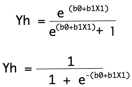
Here we can conclude that the output in defined by Yh will always be a real number between 0 and 1 which will be rounded to a integer value and mapped to a predicted class value.
Each column in our data will be associated with the coefficient (b,b1..etc) which will be learnt during the training and needs to be stored for future value predictions.
Let’s take an example with 10 samples. Here we define 10 samples of data with two features each and one label. It’s a data representing two classes which are represented by 0 and 1. Each sample is assigned with a label as 0 or 1 defined in 3rd column.
import numpy as np
data = np.array([[3.87,2.65,0],
                 [2.64,3.63,0],
                 [4.93,5.50,0],
                 [2.83,2.95,0],
                 [4.07,4.00,0],
                 [8.27,3.57,1],
                 [6.36,3.09,1],
                 [7.99,2.97,1],
                 [9.76,1.42,1],
                 [8.76,4.60,1]])
print(data)
#Output--- [[3.87 2.65 0. ] [2.64 3.63 0. ] [4.93 5.5 0. ] [2.83 2.95 0. ] [4.07 4. 0. ] [8.27 3.57 1. ] [6.36 3.09 1. ] [7.99 2.97 1. ] [9.76 1.42 1. ] [8.76 4.6 1. ]]
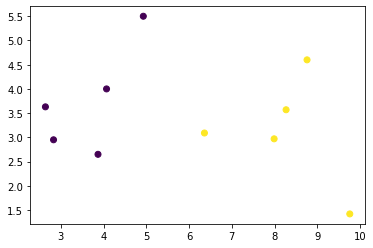
Make a plot of it on X and Y coordinates as follow. It will show two categories and two separate colors.
import matplotlib.pyplot as plt
plt.scatter(data[:,0:1],data[:,1:2],c = data[:,2:3])
plt.show()
Mathematics of Logistic Regression
Let’s define a function to calculate output using logistic regression equation.Here yhat will be first calculated as as b0 + b1x1 + b2x2 , and then the function will return the output by using yhat into logistic equation using natural logarithm.
from math import exp

# Make a prediction with coefficients
def predict(row, coefficients):
	yhat = coefficients[0]
	for i in range(len(row)-1):
		yhat += coefficients[i + 1] * row[i]
	return 1.0 / (1.0 + exp(-yhat))
We will trigger this function with data having as follows: –
coef = [0.55, 0.45, 1.10]
for row in data:
	yhat = predict(row, coef)
	print("Expected=%d, Predicted=%.3f [%d]" % (row[-1], yhat, round(yhat)))
We had defined some random coefficient to initialise the process. coef[0] is the initial bias value and coef[1] and coef[2] are coefficients values. Using initial bias and coefficient we are getting following Predicted labels which are rounded up to nearest integer value.
Expected=0, Predicted=0.995 [1]
Expected=0, Predicted=0.997 [1]
Expected=0, Predicted=1.000 [1]
Expected=0, Predicted=0.994 [1]
Expected=0, Predicted=0.999 [1]
Expected=1, Predicted=1.000 [1]
Expected=1, Predicted=0.999 [1]
Expected=1, Predicted=0.999 [1]
Expected=1, Predicted=0.999 [1]
Expected=1, Predicted=1.000 [1]
Out of total 10 samples we are having 5 predictions correct represented by 1 as expected and predicted are same. But first 5 predictions are incorrect which are expected 0 but predicted 1. So, Next process is to calculate the error value and apply error optimisation to rectify the same. The coefficients leading to minimum error value will be stored for future value predictions.
The error optimisation process to be used is Stochastic Gradient Descent which will be explained below.
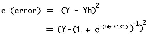
As we know we are defining the predicted output with Yh which can be represented as:

Our real output value will be defined as Y. Which leads to square of error as mentioned below.
Now we need to tune the coefficient b1 in such a way that error can becomes as minimum as possible. We can finish up this process by stochastic gradient descent. i.e we need to partially differentiate error value with respect to coefficient b1 to initiate the convergence.
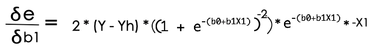
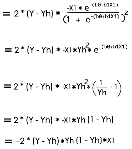
So, we figured out our gradient which can be used over coefficient b1 to converge the error value towards minimum. It is mentioned below with learning rate to regulate the learning processes.
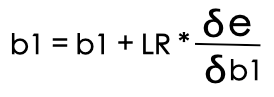
Which turned out to be a equation as mentioned below for error optimisation using Stochastic Gradient Descent.
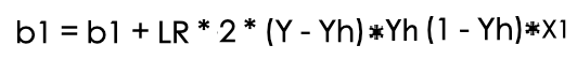
Now we can put this thing into python code to calculate coefficient values at minimum possible error. While tuning the bias or first coefficient we will not use any feature value along with gradient.
# Estimate logistic regression coefficients using stochastic gradient descent
def coefficients_sgd(train, l_rate, n_epoch):
	coef = [0.0 for i in range(len(train[0]))]
	for epoch in range(n_epoch):
		sum_error = 0
		for row in train:
			yhat = predict(row, coef)
			error = row[-1] - yhat
			sum_error += error**2
			coef[0] = coef[0] + l_rate * error * yhat * (1.0 - yhat)
			for i in range(len(row)-1):
				coef[i + 1] = coef[i + 1] + l_rate * error * yhat * (1.0 - yhat) * row[i]
		print('epoch=%d, lrate=%.3f, error=%.3f' % (epoch, l_rate, sum_error))
	return coef
Now trigger the coefficients_sgd function as mentioned below to tune our coefficients.
for row in data:
	yhat = predict(row, coef)
	print("Expected=%.3f, Predicted=%.3f [%d]" % (row[-1], yhat, round(yhat)))
#Output epoch=0, lrate=0.300, error=2.355 epoch=1, lrate=0.300, error=2.142 epoch=2, lrate=0.300, error=1.555 epoch=3, lrate=0.300, error=1.245 epoch=4, lrate=0.300, error=1.074 . . . epoch=95, lrate=0.300, error=0.100 epoch=96, lrate=0.300, error=0.098 epoch=97, lrate=0.300, error=0.097 epoch=98, lrate=0.300, error=0.096 epoch=99, lrate=0.300, error=0.095
As output you will see the error converging towards minimum possible value which was initially 2.355.
The update value of coefficients can be called as follows.
print(coef)
[-1.2764743653675956, 1.7436336944686017, -2.4845855816811415]
You can make the predictions as done below and this time you see with updated coefficients values the categories had been well classified into two groups. with no error. So we can say that the machine got trained in terms of coefficients for making out predictions using Logistic Regression.
for row in data:
	yhat = predict(row, coef)
	print("Expected=%.3f, Predicted=%.3f [%d]" % (row[-1], yhat, round(yhat)))
Expected=0.000, Predicted=0.247 [0] Expected=0.000, Predicted=0.003 [0] Expected=0.000, Predicted=0.002 [0] Expected=0.000, Predicted=0.025 [0] Expected=0.000, Predicted=0.016 [0] Expected=1.000, Predicted=0.986 [1] Expected=1.000, Predicted=0.894 [1] Expected=1.000, Predicted=0.995 [1] Expected=1.000, Predicted=1.000 [1] Expected=1.000, Predicted=0.929 [1]
Using Library–
Scikit-Learn provides us a library support to implement Logistic regression in easier way. Let’s have a look. We will use Pima India Diabetic Dataset.
import pandas as pd
df = pd.read_csv('diabetes.csv')

X = df.drop(['Outcome'],axis=1)
Y = df['Outcome']

from sklearn.model_selection import train_test_split
xtrain,xtest,ytrain,ytest = train_test_split(X,Y)

from sklearn.linear_model import LogisticRegression
lmodel = LogisticRegression()

lmodel.fit(xtrain,ytrain)

print('Training Accuracy:',lmodel.score(xtrain,ytrain))
print('Testing Accuracy:',lmodel.score(xtest,ytest))
Training Accuracy: 0.7743055555555556 Testing Accuracy: 0.7239583333333334
So at the end we are getting 77% training and 72% Testing accuracy on diabetic data with 8 features of a person and label representing Diabetic or Non-Diabetic.
Now we can get our final coefficients as follows. Since we are having 8 features so 8 coefficients are generated and one bias value.
print(lmodel.coef_)
print(lmodel.intercept_)
[[ 0.14515144 0.04110736 -0.01092623 -0.00195708 -0.00125506 0.09054463 0.12483913 0.00827183]]

[-8.76810019]
To make predictions on some unknown value we will apply .predict function as follow.
status = np.array(['Non - Diabetic' , 'Diabetic'])
print(status[lmodel.predict(xtest.iloc[45:46,:])])
['Diabetic']
So we concluded logistic regression can be used in two categorical predictions mathematically or by using Scikit-Learn Library. You can choose your way of coding.
Thanks for being a Patience Learner. Keep Learning… Good luck