Eigenvector represents greatest variance in case of PCA
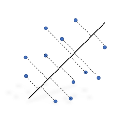
In case of Principal Component Analysis we project our data points on a vector in a direction of maximum variance to decrease the number of existing components. In this case we consider the direction eigenvector generated using covariance matrix as the direction of maximum variance. In this article we look into the proof of why eigenvector is considered as direction of maximum variance.
Mean of vector projection on Eigen vector.
Suppose there is a eigenvector as follows and x1, x2 and x3 are the points projected over it. Then the scaler projection of points can be represented as mentioned below using Xz.

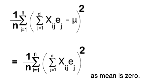
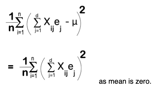
Mean of all the points projected can be represented as: –

Here, the mean of term Xij is 0 as normalised data is being used for projection whose mean used to be zero. It signifies that mean of all projected value on a Eigen Vector is Zero.
Variance of Projected Points is the Eigenvalue
Variance of points projected on Eigen Vector can be represented as: –
Variance =
Now we can write a similar equation by breaking the square term and using two sums with attributes j and a. These two sums will be exactly identical i.e. j = a.

Now we will rearrange the equation by grouping all the term with i.

We can easily identify the term inside the bracket as Covariance matrix between component j and I and can be represented as: –

Now we know that the multiplication of an Eigenvector with covariance matrix can be represented by a scaler value (ג) multiplication with eigenvector. i.e.

So, We can rewrite our variance as: –

Since, Eigenvector (e) we consider as unit vector so its magnitude will be one and variance will be equal to ג, Which is the Eigenvalue.
So it is concluded that the variance of projection is same as Eigenvalue of the Eigenvector considered.
The only way to Learn Mathematics is to do mathematics.
Paul Halmos
Eigen Vector = Greatest Variance
Eigenvector gives you the dimension of greatest variance. Suppose e is any vector and we need to project Xi points on e. Then we will measure the variance of the projections.
The projections are done by dot products so, we will do dot products between x1 and e, x2 and e and so on…. So we will get a scaler number which will represent where the projection over e.
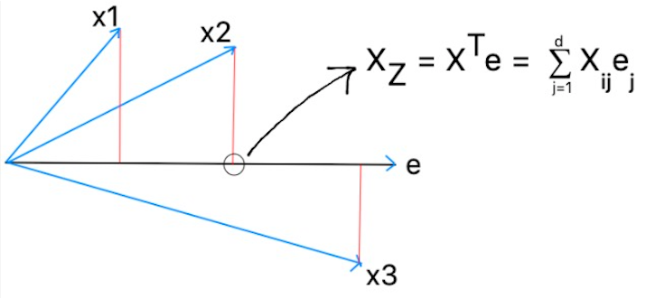
When we will have just number we can easily measure variance. So measure of variance can be defined as: –
Variance =
Now we want make this variance as big as possible i.e. we need to take vector e in such a way that variance V becomes as big as possible.
When we have a formula which is differentiable we take the derivative and set it equals to 0 and solve it to get into a point of highest value condition.
In this case we can’t directly do that as we had assumed e as a vector not eigenvector which can be turned into a very big value to make variance large. So we will end up as a huge value of e which is not needed.
So we will put a constraint to control it and make sure that e turns out to be a unit vector i.e. we will cap the length of vector e such that ||e|| = 1. We will add a lagrange multiplier so that solution can be a unit length for e.
Take the length of e use ג as coefficient or lagrange multiplier.

Now we can take the derivative and set the derivative to zero. Differentiate with the component of e i.e. value of e for attribute a.
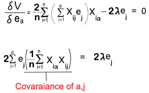
So, after rearranging the equation we end up with a equation where one term of LHS is representing the covariance as below.
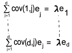
Here what we are doing ? We are summing up over the J’s using dot product between vector e and first row of covariance matrix because this is the set of Covariances with the first attribute and its the first row of matrix which we are multiplying with by vector e.
It gives us first row of matrix times the vector e is the first component of vector e multiplied by a lagrange multiplier and so on till the last which represents last row of matrix times the vector e is the last component of vector e multiplied by a lagrange multiplier.
So we can say that we are taking rows of a covariance matrix multiplying by a vector e and we get the same vector back multiplied by any coefficient ג. When we will put it all together we will get the following equation.

What this equation is telling to us ? It says e must be a Eigenvector. Thus we can say that eigenvector represents dimensions of greatest variance. And the coefficient ג is a eigenvalue.
How many Components ?
When we do eigen decomposition we end of with as many Eigen vectors components as we have original dimensions. So for d cordite d eigenvectors will be generated. To reduce dimensionality to choose m which is smaller than d i.e. m < d. As eigen value is representation of variance so we will take the maximum one first but how do we know when to stop.
We follow certain procedure as follow: –
a. Sort eigenvectors using eigenvalue such that
𝝺1 >= 𝝺2 >= 𝝺3 >= 𝝺4 >=……..>= 𝝺d
b. Pick first m vectors which represents 90% to 95% of total variances. If we add up first m Eigenvalues and divide by sum of all Eigenvalues we will get what proportion of information or variances stored by those m eigenvectors.
If we plot the cumulative sum of the eigenvalue it will give a shape as drawn below: –
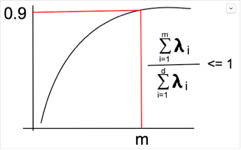
With first few eigenvectors we can capture maximum of variances but to reach 100% we have to consider many many vectors. So we pick upto 90% to 95% of variances using first m vectors which satisfies it.
Second way of doing it is by plotting scree plot. Here we plot eigenvalue on y-axis and number of dimensions associated on x axis as shown below.
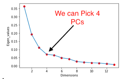
We can choose stoping point 4 in this case after which the eigenvalues turns out to be stiffer and can represent around 90% of the variances.

