
Mean, Variance, Standard Deviation, Standard Score, Covariance & Data Projection
Variance – It is the measure of squared difference from the Mean. To calculate it we follow certain steps mentioned below:
- Calculate average of numbers
- For each numbers subtract the mean and square the result
- Calculate the average of those squared differences i.e. Variance
Example: –
Suppose you have weights of 5 different persons as [88 , 34 , 56 , 73 , 62]. You need to find out Mean, Variance and Standard Deviation.
Mean = (88 , 34 , 56 , 73 , 62)/5 = 62.6
Variance, Average of square of differences.
Variance = ((25.4)2 + (10.4)2 + (-28.6)2 +(-6.6)2 + (-0.6)2) / 5 = 323.04
Standard Deviation, Square root of Variance
Standard Deviation = (323.05)1/2 = 17.97

So, With Standard deviation we figure out the “standard” way of knowing what is normal in data and what are extra large or small values. Like in this case having a weight of 88 or 34 is extra large or too small as compared to other entities.
We can expect around 68% of values within plus or minus of standard deviation.
Here 3 out of 5 data points are within 1 standard deviation i.e. 17.97 and 5 out of 5 are within 2 standard deviation i.e. 17.97*2 = 35.94
In General what we figure out from the concept pf standard deviation is as follow-
- likely to be within 1 standard deviation (68 out of 100 sample points)
- very likely to be within 2 standard deviation (95 out of 100 sample points)
- almost certainly to be within 3 standard deviation (97 out of 100 sample points)
Standard Score or Standardization
Standardization is process of generating standard normal distribution of data. We need to first transform the data in a way that its mean becomes 0 and standard deviation is 1. Steps are as follows-
- First subtract the mean
- Then divide by standard deviation

z = standard score
x = value to be standardised
µ = mean of data points
σ = standard deviation
Why Standardize ?
Standardization helps in making decisions about a set of data by creating uniform distribution around the mean.
Example: – Suppose there is a test conducted and students get marks out of 50 as follows-
22,17,28,30,20,26,37,16,26,22,19
Most of the student are below 25 so most will fail as per conventional assumptions.
As test is quite hard so decision can be made using standardise data by failing those who are 1 standard deviation below the mean.
Here the mean is 24 and standard deviation is 5.96, which results into following standard score.
-0.33, -1.17 , 0.67, 1.00, -0.67 , 0.33 , 2.18 , -1.34 , 0.33, -0.33, -0.83
The information that we gather are following-
- Out of total 11 samples 7 are within 1 standard deviation 10 are within 2 standard deviation and 11 i.e. all samples are within 3 standard deviation.
- Only two student will fail with standard score -1.17 and -1.34 as they are below the mean by standard deviation 1.
This process makes calculation much easier as we need only one table which is Standard normal distribution, rather than individual calculations for each value of mean and standard deviation.
Covariance
Suppose we are having data sample with 3 features than Covariance matrix show how similar the variances of the features are ?
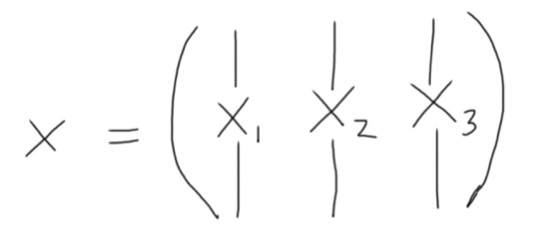
Our data samples represented by X with 3 features x1, x2, x3. The features had been transformed in a way that their mean becomes zero. i.e. x1 = x1 – mean(x1), x2 = x2 – mean(x2), x3 = x3 – mean(x3) standard normal distribution.
Now we need to calculate covariance matrix using X which is the similarity between the features. We know to figure out similarity we can use dot product. We can represent the procedure as follow.

The matrix generated is meant to give us certain information as listed below.
- (XTX)ij represents similarity of change of ith and jth feature but using this procedure will let us deal with huge number as dimension increases.
- So, we divide it by n to solve the problem, which gives us result like below:

Cov(X) = (XTX) / n
It shows that ith and jth row of a covariance matrix shows the co(variance) of the ith and jth features
Let’s take an example to understand it.
Suppose there are two stocks A and B and we are having data of their daily return as follows.
| Day | Return of A | Return of B |
| 1 | 1.1% | 3.0% |
| 2 | 1.7% | 4.2% |
| 3 | 2.1% | 4.9% |
| 4 | 1.4% | 4.1% |
| 5 | 0.2% | 2.5% |
Now we will calculate the average return of each stock.
Average, A = (1.1+1.7+2.1+1.4+0.2) / 5 = 1.30
Average, B = (3+4.2+4.9+4.1+2.5) / 5 = 3.74
To calculate covariance, we take take products differences between return of A and the average calculated and the difference of B from its average calculated.
i.e. Covariance = ∑((Return of A – Average of A) * (Return of B – Average of B)) / Sample size
= ([(1.1 – 1.30) * (3 – 3.74)] + [(1.7 – 1.30) * (4.2 – 3.74)] + [(2.1 – 1.30) * (4.9 – 3.74)] + ……)/5
= 2.66 / 5
= 0.53
The Covariance calculated is a positive number which indicates both returns are in same direction. i.e. When A is having high return B is also having a high return.
Example of Covariance and Scaling: – Consider a data with two features defined as x and y as follow.
import numpy as np
import matplotlib.pyplot as plt

plt.style.use('ggplot')

# Normal distributed x and y vector with mean 0 and
# standard deviation 1
x = np.random.normal(0, 1, 500)
y = np.random.normal(0, 1, 500)
X = np.vstack((x, y)).T

plt.scatter(X[:, 0], X[:, 1], color = 'red')
plt.title('Generated Data')
plt.axis('equal')
plt.show()
# Covariance
def cov(x, y):
    xbar, ybar = x.mean(), y.mean()
    return np.sum((x - xbar)*(y - ybar))/(len(x) - 1)

# Covariance matrix
def cov_mat(X):
    return np.array([[cov(X[0], X[0]), cov(X[0], X[1])], \
                     [cov(X[1], X[0]), cov(X[1], X[1])]])

print(cov_mat(X.T))
[[ 0.9904346 , -0.04658066], [-0.04658066, 0.83919946]]
It shows covariances of column x and y. Now we well transform our data to make it uncorrelated by using a scaling matrix as mentioned below.
# Center the matrix at the origin
X = X - np.mean(X, 0)

# Scaling matrix
sx, sy = 5, 1
Scale = np.array([[sx, 0], [0, sy]])

print(Scale)
#Output

[[5, 0],
 [0, 1]]
# Apply scaling matrix to X
Y = X.dot(Scale)
plt.figure(figsize=(9,6))
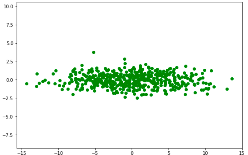
plt.scatter(Y[:, 0], Y[:, 1],color='green')
plt.title('Transformed Data')
plt.axis('equal')
# Calculate covariance matrix
print(cov_mat(Y.T))
The Covariance matrix of transformed data shows that x and y are now uncorrelated with Covariance values close to zero and variance for x and y are enhanced upto 24.76 and 0.839.
Introduction to Projection of Vector
Suppose there is a Line L and and vector X needs to be projected over L. Then vector on L represented by perpendicular from vector X on L is known as projection of Vector X over L i.e. Some vector in L where [vector(X) – Proj L V(X)] is orthogonal to L.

Scaler Projection of a Vector

Vector Projection over a Line
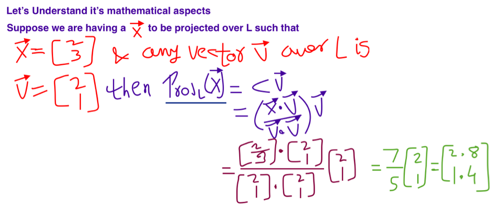
Here the magnitude of projection is 7/5 over the line L and the direction of projection will be observed by vector [2.8 , 1.4].
Note: – In case of PCA we use magnitude of projection over eigenvector.
For Detailing of Eigenvector and Eigenvalues Click Here