
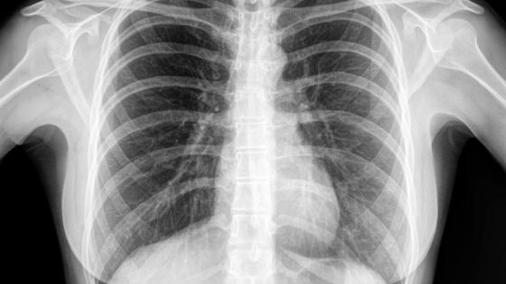
Convolutional Neural Network model to identify PNEUMONIA using Chest X-Ray images.
Here we will develop a deep learning model using CNN VGG-16 architecture to predict about Pneumonia using any chest x-ray image with more then 95% of accuracy.
With continuous growth in the field of AI and Machine Learning It is stepping into almost every section of industry. In healthcares sector a lot of analysis can be done using Machine Learning over patients health report and prediction can be made about the type of infection he can develop or is already suffering from.
In this discussion we will use chest X-ray of around 5k persons. Out of complete data set around 3800 are representing Pneumonia patient and 1341 are representing normal persons X-ray. We need to develop a model in such a way that it can be easily predicted by a machine using the chest X-ray image that whether a person is healthy or not.
Source of Data: – Chest X-Ray Images
We will Start by importing the library need to develop a CNN model. We will be using Keras which is one of very powerful library used in deep learning for neural networks.
import keras
from keras.models import Sequential
from keras.utils import np_utils
from keras.preprocessing.image import ImageDataGenerator
from keras.layers import Dense, Activation, Flatten, Dropout, BatchNormalization
from keras.layers import Conv2D, MaxPooling2D
from keras import regularizers
from keras.callbacks import LearningRateScheduler
import numpy as np
We can use a decaying learning rate and to use it we need to define a decay rate as follows: –
def lr_schedule(epoch):
    lrate = 0.001
    if epoch > 75:
        lrate = 0.0005
    if epoch > 100:
        lrate = 0.0003
    return lrate
For supervised learning we need dependent and independent variables. So we can use the name or directory of images to generate separate labels for separate images. Here for all images present in directory NORMAL we added 0 into the list declared as labels and for all images in the directory PNEUMONIA we added 1 as label. So we are having two categorical value 0 and 1 representing two types of person.
import os
labels = []
for i in os.listdir('../input/chest-xray-pneumonia/chest_xray/train/NORMAL'):
    labels.append(0)
for i in os.listdir('../input/chest-xray-pneumonia/chest_xray/train/PNEUMONIA'):
    labels.append(1)
For dependent variable we will extract feature of all the images using computer vision and store them as features.
import cv2
loc1 = '../input/chest-xray-pneumonia/chest_xray/train/NORMAL'
loc2 = '../input/chest-xray-pneumonia/chest_xray/train/PNEUMONIA'
features = []
from tqdm import tqdm
for i in tqdm(os.listdir(loc1)):
    f1 = cv2.imread(os.path.join(loc1,i))
    f1 = cv2.resize(f1,(100,100))
    features.append(f1)

for i in tqdm(os.listdir(loc2)):
    f2 = cv2.imread(os.path.join(loc2,i))
    f2 = cv2.resize(f2,(100,100))
    features.append(f2)
Next we need to normalise the data and to do it we will convert the data into Numpy array. After normalisation divide the data into training and testing sets. The training samples will be used to impart training to our model and testing samples will be used for evaluating our model performance on unknown set of data inputs.
import numpy as np
Y = np.array(labels)
X = np.array(features)

#Normalisation of features
Xt = (X - X.mean())/X.std()
Yt = np_utils.to_categorical(Y)

#Seperating training and validation set
from sklearn.model_selection import train_test_split
x_train,x_test,y_train,y_test = train_test_split(Xt,Yt)
Develop a VGG-16 CNN model as shown below to make the predictions.
weight_decay = 1e-4
model = Sequential()
model.add(Conv2D(32, (3,3), padding='same', kernel_regularizer=regularizers.l2(weight_decay), input_shape=x_train.shape[1:]))
model.add(Activation('elu'))
model.add(BatchNormalization())
model.add(Conv2D(32, (3,3), padding='same', kernel_regularizer=regularizers.l2(weight_decay)))
model.add(Activation('elu'))
model.add(BatchNormalization())
model.add(MaxPooling2D(pool_size=(2,2)))
model.add(Dropout(0.2))

model.add(Conv2D(64, (3,3), padding='same', kernel_regularizer=regularizers.l2(weight_decay)))
model.add(Activation('elu'))
model.add(BatchNormalization())
model.add(Conv2D(64, (3,3), padding='same', kernel_regularizer=regularizers.l2(weight_decay)))
model.add(Activation('elu'))
model.add(BatchNormalization())
model.add(MaxPooling2D(pool_size=(2,2)))
model.add(Dropout(0.3))

model.add(Conv2D(128, (3,3), padding='same', kernel_regularizer=regularizers.l2(weight_decay)))
model.add(Activation('elu'))
model.add(BatchNormalization())
model.add(Conv2D(128, (3,3), padding='same', kernel_regularizer=regularizers.l2(weight_decay)))
model.add(Activation('elu'))
model.add(BatchNormalization())
model.add(MaxPooling2D(pool_size=(2,2)))
model.add(Dropout(0.4))

model.add(Flatten())
model.add(Dense(2, activation='softmax'))

model.summary()
Output: –
Model: "sequential"
_________________________________________________________________
Layer (type)                 Output Shape              Param #
=================================================================
conv2d (Conv2D)              (None, 100, 100, 32)      896
_________________________________________________________________
activation (Activation)      (None, 100, 100, 32)      0
_________________________________________________________________
batch_normalization (BatchNo (None, 100, 100, 32)      128
_________________________________________________________________
conv2d_1 (Conv2D)            (None, 100, 100, 32)      9248
_________________________________________________________________
activation_1 (Activation)    (None, 100, 100, 32)      0
_________________________________________________________________
batch_normalization_1 (Batch (None, 100, 100, 32)      128
_________________________________________________________________
max_pooling2d (MaxPooling2D) (None, 50, 50, 32)        0
_________________________________________________________________
dropout (Dropout)            (None, 50, 50, 32)        0
_________________________________________________________________
conv2d_2 (Conv2D)            (None, 50, 50, 64)        18496
_________________________________________________________________
activation_2 (Activation)    (None, 50, 50, 64)        0
_________________________________________________________________
batch_normalization_2 (Batch (None, 50, 50, 64)        256
_________________________________________________________________
conv2d_3 (Conv2D)            (None, 50, 50, 64)        36928
_________________________________________________________________
activation_3 (Activation)    (None, 50, 50, 64)        0
_________________________________________________________________
batch_normalization_3 (Batch (None, 50, 50, 64)        256
_________________________________________________________________
max_pooling2d_1 (MaxPooling2 (None, 25, 25, 64)        0
_________________________________________________________________
dropout_1 (Dropout)          (None, 25, 25, 64)        0
_________________________________________________________________
conv2d_4 (Conv2D)            (None, 25, 25, 128)       73856
_________________________________________________________________
activation_4 (Activation)    (None, 25, 25, 128)       0
_________________________________________________________________
batch_normalization_4 (Batch (None, 25, 25, 128)       512
_________________________________________________________________
conv2d_5 (Conv2D)            (None, 25, 25, 128)       147584
_________________________________________________________________
activation_5 (Activation)    (None, 25, 25, 128)       0
_________________________________________________________________
batch_normalization_5 (Batch (None, 25, 25, 128)       512
_________________________________________________________________
max_pooling2d_2 (MaxPooling2 (None, 12, 12, 128)       0
_________________________________________________________________
dropout_2 (Dropout)          (None, 12, 12, 128)       0
_________________________________________________________________
flatten (Flatten)            (None, 18432)             0
_________________________________________________________________
dense (Dense)                (None, 2)                 36866
=================================================================
Total params: 325,666
Trainable params: 324,770
Non-trainable params: 896
_________________________________________________________________
Apply data argumentation to boost up the data variance. This process is very helpful if our data samples are less and we need to train our model on more number of data with more variations in the features.
#data augmentation
datagen = ImageDataGenerator(
    rotation_range=15,
    width_shift_range=0.1,
    height_shift_range=0.1,
    horizontal_flip=True,
    )
datagen.fit(x_train)
Train your model using the features value extracted. The training will done for 30 times and accuracy will be monitored continously.
#training
batch_size = 64

adam = keras.optimizers.Adam(lr=0.001,decay=1e-6)
model.compile(loss='categorical_crossentropy',
              optimizer=adam, metrics=['accuracy'])
model.fit_generator(datagen.flow(x_train, y_train,
                                 batch_size=batch_size),
                    steps_per_epoch=x_train.shape[0] // batch_size,
                    epochs=30,verbose=1,
                    validation_data=(x_test,y_test),
                    callbacks=[LearningRateScheduler(lr_schedule)])
#save to disk
model_json = model.to_json()
with open('model.json', 'w') as json_file:
    json_file.write(model_json)
model.save_weights('model.h5')
#Training ---
Epoch 25/30
61/61 [==============================] - 12s 190ms/step - loss: 0.1855 - accuracy: 0.9589 - val_loss: 0.3214 - val_accuracy: 0.9233 - lr: 0.0010
Epoch 26/30
61/61 [==============================] - 13s 218ms/step - loss: 0.2207 - accuracy: 0.9480 - val_loss: 0.3021 - val_accuracy: 0.9333 - lr: 0.0010
Epoch 27/30
61/61 [==============================] - 12s 192ms/step - loss: 0.1949 - accuracy: 0.9574 - val_loss: 0.1370 - val_accuracy: 0.9739 - lr: 0.0010
Epoch 28/30
61/61 [==============================] - 12s 189ms/step - loss: 0.1703 - accuracy: 0.9628 - val_loss: 0.1461 - val_accuracy: 0.9716 - lr: 0.0010
Epoch 29/30
61/61 [==============================] - 12s 193ms/step - loss: 0.1633 - accuracy: 0.9654 - val_loss: 0.4172 - val_accuracy: 0.8911 - lr: 0.0010
Epoch 30/30
61/61 [==============================] - 12s 189ms/step - loss: 0.1870 - accuracy: 0.9540 - val_loss: 0.2418 - val_accuracy: 0.9402 - lr: 0.0010
After 30 training epochs we reached at a point where training accuracy is around 95% and then we need to evaluate testing accuracy as follows.
#testing
scores = model.evaluate(x_test, y_test, batch_size=128, verbose=1)
print('\nTest result: %.3f loss: %.3f' % (scores[1]*100,scores[0]))
11/11 [==============================] - 0s 27ms/step - loss: 0.2418 - accuracy: 0.9402 Test result: 94.018 loss: 0.242
This shows our validation accuracy is 94% i.e. accuracy in prediction on unknown x-ray images our model is predicting with almost 94% accuracy. Which signifies model is not overfit.
We choose any random value for prediction as follow.
status = np.array(['Normal' , 'Pneumonia'])
prediction = np.argmax(model.predict(x_test[503].reshape(1,100,100,3)))
print('Actual Label:',np.argmax(y_test[503]))
print('Predicted Value:',prediction)
print('Predicted Label:',status[prediction])

import matplotlib.pyplot as plt
plt.imshow(x_test[503])
plt.show()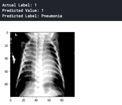
You can try with some other sets of images and to train your model and make predictions. Comment down your querries.
Thanks for your reading. Suggestions are always welcome. Keep Learning…